Exploratory Data Analysis (EDA) on Wine Quality Prediction Dataset

1. Introduction

The article consists of Exploratory Data Analysis (EDA), predictive models and evaluation of those models for predicting the quality of wine, given a list of wine characteristics.

Note: Dataset and code can be found here.

2. Problem Specification

The dataset specifies the quality of wine, given a list of attributes. The attributes are fixed acidity, volatile acidity, citric acid, residual sugar, chlorides, free sulfur dioxide, total sulfur dioxide, density, pH, sulphates, alcohol, and type (0 for red wine, 1 for white wine). These attributes are also known as feature set of a dataset. Along with these features, we have a label for each entry of the data, the quality of the wine which is basically a score between 0 and 10.

Now, given those features and label, we have to predict the quality of wine for some unknown set of data (test data) where the quality is not given.

3. Exploratory Data Analysis (EDA)

EDA is used for seeing what the data can tell us beyond the formal modeling or hypothesis testing task [1]. Before fitting into models, we explore the data to have a broader impression of the data.

3.1 Summary of the Features

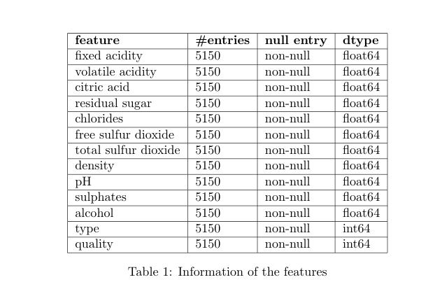
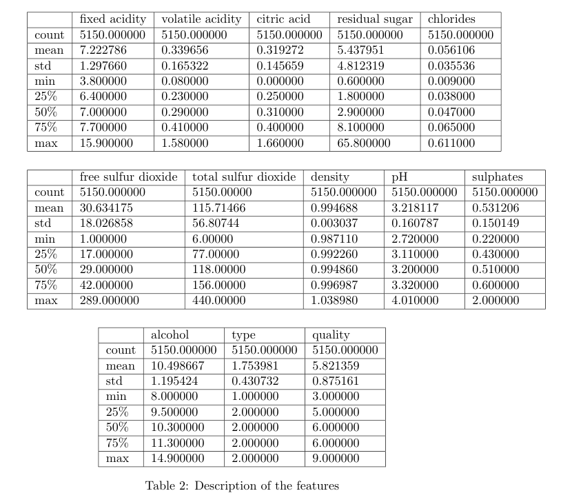
Table 1 shows the basic information about the feature columns. Here, we can see that there is no null or missing value in the data, since each column has the same number (5150) of entries. Also, we can see that other than our label column quality, we have type column which is of integer data type. Now, let’s look at the summary of the data for each feature. Table 2 shows us minimum, maximum, mean and quartile information of the data for each feature.

3.2 Univariate Analysis

We want to see how the data is distributed for each feature. When we only look at the distribution of the data within a single feature, we call it univariate analysis. Let’s look at the figure 1 that depicts univariate histogram plot for each feature. We can observer that

• wine quality is approximately normally distributed
• the pH is normally distributed, with few outliers
• fixed acidity have some outliers and peaks between 6 and 7
• volatile acidity has quite a few outliers with high values, also slightly skewed to the right
• most of the wines have citric acid within the range of 0.25-0.30 with few other spikes at 0.01 and 0.48
• density has almost normal distribution
• there are many outliers with high residual sugar and the distribution is skewed right
• chloride distribution is skewed right with outliers.
• distribution of free sulfur dioxide and total sulfur dioxide is skewed right
• the feature type seems to be ordinal or categorical data with numeric representation

Figure 1: Histogram plots of the dataset

Since the type feature is ordinal, there are chances that it could externally affect the distribution of other features. Let’s find the information of the dataset for each value of type, and observe if it shows any changes in the distribution. Figure 2 depicts the changes in the distribution of each feature for two different values of feature type.

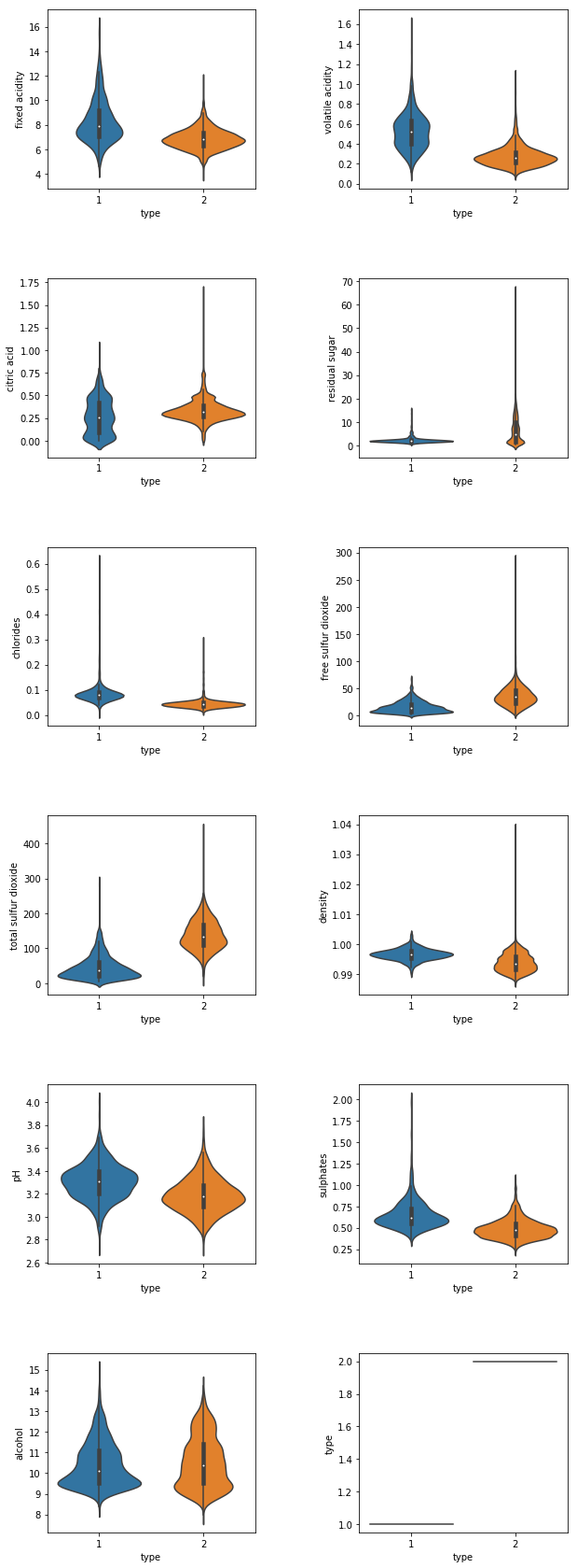Figure 2: Violin plots of two different type of wines

3.3 Bivariate Analysis

Here, we will analyze correlations between each feature with other features. This will help us finding similar or related features by only visual inspection.

Figure 3 shows the correlations between each pair of features in heatmap style. We can observe that residual sugar has a noticeable positive correlation with density. Also total sulfur dioxide is strongly correlated with the type of wine.

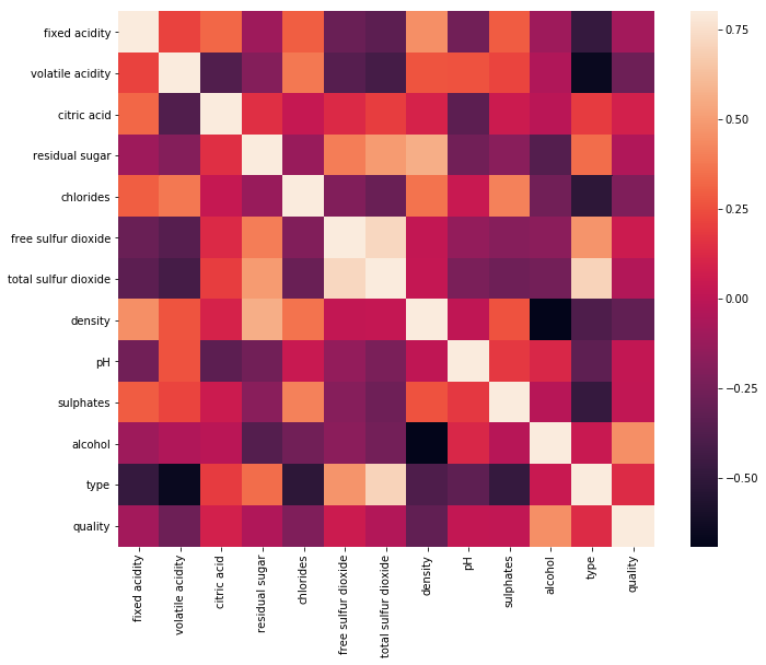Figure 3: Heatmap style correlation matrix

Now, let’s have a closer look at the sorted version of the heatmap with respect to quality in the figure 4. We can easily figure out that, the amount of alcohol seems to be the most correlated feature for determining the quality of wine.

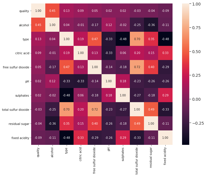Figure 4: Heatmap style correlation matrix sorted w.r.tquality

Pairwise scatter plots give us more insight about the correlation with a different visualization perspective. Figure 5 shows pairwise scatter plots of the dataset.

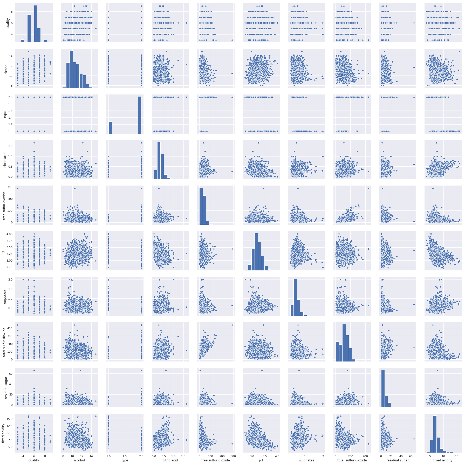Figure 5: Pairwise scatter plots

4. Data Preprocessing

4.1 Finding Missing Values

From the table 1, we can confirm that there are no missing values in this dataset.

4.2 Split Dataset

We find from the EDA that the feature type is ordinal and affects almost all features, so we split the dataset into two, one with type 1 and other with type 2.

4.3 Outliers Removal

There are several outliers detection methods. We applied Inter Quartile Range (IQR) method to remove outliers.

4.4 Feature Selection

We applied SelectKBest with chi2 scoring function from sklearn [2] and found that volatile acidity, citric acid, free sulfur dioxide, total sulfur dioxide, and alcohol are the top five features for this dataset.

We also applied Recursive Feature Selection using logistic regression and Extra Trees Classifier for finding the best useful features for determining the quality of wines.

Observing the results from feature selection methods, we select alcohol, total sulfur dioxide, sulphates, volatile acidity, density, residual sugar, chlorides, pH, and free sulfur dioxide as features for type 1 wines and alcohol, volatile acidity, density, free sulfur dioxide, total sulfur dioxide, residual sugar, sulphates, and chlorides for type 2 wines.

5. Modeling Classifier

We can find the solution using a regression model since the outcomes range from 3 to 9, as well as classification model since we can define the outcomes as some certain classes.

We design both kinds of models, and find that only tree based classifiers perform well, particularly Extra Trees classifier and Random Forest classifier outperform all other existing kinds of regressors and classifiers. For type 1 wines, Random Forest Classifier gives the best MAE and for type 2 wines, Extra Trees Classifier gives the best MAE. Parameters for both types are given below:

• number of estimators=500
• min samples leaf=1

We can observe the Cross Validation Mean (CVM) and MAE scores in the table 3.

6. Conclusion

We experiment with different types of classification and regression models for this task. The best MAE score we find with this dataset is 0.336819. There are still plenty of scopes to experiment with the data, specially in depth exploratory data analysis could help understand the data more accurately.

7. References

[1] EDA - Wikipedia: https://en.wikipedia.org/wiki/Exploratory_data_analysis

[2] sklearn: https://scikit-learn.org