Introduction

Point clouds are a collection of data points in space, usually produced by a 3D scanner. A large number of points are measured on the external surfaces of the objects and then represented as point clouds. Along with the relative 3D coordinates, point clouds can be accompanied by other pertaining features i.e. RGB or intensity. Point clouds are not the only representation of 3D space, voxel and mesh polygon are some other popular representations. Figures 1, 2, and 3 are some examples of different 3D space representations.

Fig. 1: Example of point cloud representation [4]

Fig. 2: Example of voxel representation [5]

Fig. 3: Example of polygon mesh representation [6]

Fast acquisition of 3D point cloud from sensor devices has been exhilarating researchers to concentrate on processing these raw data directly, rather doing any kind of preprocessing. Consequently, there is a set of applications built on point cloud processing including navigation [7], self-driving [8], robotics [9], shape synthesis and digital modeling [10].

Fitting raw point cloud data into deep learning model is not straightforward with respect to other conventional ways of doing it due to the irregular structure of point clouds. Continuous distribution of the point positions in the space and unordered set of points make it harder to extract spatial information through point clouds data. One of the pioneering works in the field of point clouds processing is called PointNet [2], which overcomes the permutation invariance issue of point cloud data. There are other extensions available inspired by this work, which try to exploit local features considering neighborhood points and resulting in improved performance.

To gain proper geometric relationships among points, the authors of the titled paper propose an operation called EdgeConv using the concepts from graph neural networks. They extend the PointNet modules by incorporating EdgeConv, which can be easily integrated into existing deep learning models. They achieve state-of-the-art performance on several datasets, including ModelNet40 and S3DIS for classification and segmentation tasks.

Related Work

There has been a pile of works pertaining to capture local feature descriptors for point clouds which are basically handcrafted features intended towards certain types of problems and intermediate data structures [11]-[13]. On top of that, machine learning approaches are wrapped around to generate end results.

With the emergence of convolutional neural networks (CNNs) [14], [15], handcrafted features are not being embraced anymore. The simplest form of a CNN architecture mixes convolutional and pooling units to accumulate the local information in images. Figure 4 shows a basic CNN architecture.

Fig. 4: A basic CNN architecture [16]

There are mainly two types of 3D deep learning methods, namely view-based and volumetric methods. While view-based methods apply standard CNNs on 2D views of the target 3D object [17], [18], conversion of geometric data to a regular 3D grid takes place before passing through a CNN in volumetric methods. Voxelization is one of the simplest ways to do the conversion [19], [20]. There are also studies on combination of both methods [21].

PointNets [2] apply a symmetric function on point clouds data to achieve permutation invariant features. PointNets treat each point individually for learning 3D latent features which is unaware of local geometric structures and to achieve the global transformation. However, the employed spatial transformer network [22] gets really complex and computationally expensive for this kind of non-Euclidean data.

PointNet++ [3] architecture is an improved version of PointNet to exploit the local geometric features. Although PointNet++ achieves state-of-the-art results on several point cloud analysis benchmarks, still it treats individual points in local point sets independently.

PointCNN [23], KCNet [24] are some other networks to improve PointNets lacking. However, all of these neglect geometric relationships among points leading to local feature missing.

Point cloud data are of non-Euclidean structure. To achieve the best results out of non-Euclidean data, geometric deep learning [25] comes into play. In [26], convolution for graphs was proposed based on Laplacian operator [27]. Although it introduces convolutional operations on graph-based data, the computational complexity of Laplacian eigendecomposition is one of the drawbacks of the proposition. To eliminate this complexity there have been some follow-up studies where different types of spectral filters [28]-[30] are used and also guarantee spatial localization.

Domain-dependent spectral graph CNNs cannot generalize a learned filter for unknown shapes. Spectral transformer networks [31] help in this regard, but not entirely. More generalization could be possible by an alternative definition of non-Eucledian spatial filters. Deep CNN on meshes, also named as Geodesic CNN (GCNN) [32] employs such filters.

Dynamic Graph CNN (DGCNN)

Graph

Graph represents a set of objects (nodes) and their relationships (edges). A lot of real-world data doesn’t fit into grids. Social networks data, knowledge graph, transportation or communication networks, protein interaction networks, and molecular networks are to name a few of the real-world data, which we need to take care of differently before passing into the neural networks. Graph neural networks can directly operate on graph structure and can be used for node classification, graph classification, link prediction, and so on. Figure 5 shows the visual difference of Euclidean grid and non-Euclidean graph data.

Fig. 5: Left- Euclidean space, Right- graph in non-Euclidean space [33]

Graph Convolution Networks (GCNs)

In GCNs, convolutional operations are applied similar to the standard CNNs, but on graph data. GCNs can be divided into two major types: spectral-based and spatial-based GCNs. Spectral-based GCNs apply filters from the perspective of graph signal processing and involve Eigen decomposition of graph Laplacian. Graph convolution operation in GCNs can be interpreted as removing noise from graph signals. Spatial-based GCNs formulate graph convolutions as aggregating feature information from neighbors.

GCNs generalize the operation of convolution from traditional data (images or grids) to graph data. They learn a function, $f$ to generate a node $v_i$ s representation by aggregating it’s own features $X_i$ and neighbors’ features $X_j$ where $j \in N(v_i)$ namely neighborhood aggregation. Figure 6 shows a simple approach to aggregate neighborhood information.

Fig. 6: Neighborhood aggregation [34]

In the ideal case, equations 1, 2, and 3 represent spatial based GCNs and show how to aggregate neighborhood information. Initially, for the first layer, embeddings are set to the equal values of node features (shown in equation 1). After that, the $k$ h layer embedding of node $v$ can be found by summing up the average of neighbors’ previous layer embeddings and previous layer embedding of $v$ followed by applying a non-linear activation function i.e. ReLU or tanh (shown in equation 2). At last, $h_v^k$ can be sent to any loss function and stochastic gradient descent will train the matrices $W_k$ and $B_k$ .

$$ h_v^0 = x_v \ \ \ \ \ (1) $$

$$ h_v^k = \sigma \left ( W_k \sum_{u \in N(v)} \frac{h_u^{k-1}}{|N(v)|} + B_kh_v^{k-1} \right ), \forall k \in {1,…,K} \ \ \ \ \ (2) $$

$$ z_v = h_v^K \ \ \ \ \ (3) $$

In GCNs, max/min/sum/average pooling can be seen as graph coarsening [35] which is responsible for creating structurally similar to the original but smaller graphs [36]. Figure 7 and 8 show the differences in basic pooling operation in grid-based CNNs and GCNs respectively.

Fig. 7: Max pooling operation in grid-based CNN [37]

Fig. 8: Graph coarsening used as pooling operation in GCN [38]

Interleaving aggregation and coarsening, one after another, figure 9 shows a generalized skeleton of a GCN.

Fig. 9: GCN with pooling layer for graph classification [39]

EdgeConv

Definition

In the titled paper, authors introduce an operation called EdgeConv which has translation-invariant and non-locality properties. It captures local geometric structures from local neighborhood graph and applies convolution-like operations on the edges. Unlike graph CNNs, the graph dynamically updates after each layer of the network.

Point clouds can be seen as graph $G=(V,E)$ where $v={1,…,n}$ and $E \subset V \times V$ In the simplest case, they construct k-NN graph in $R^F$ containing directed edges of the $(i,j_{i1}),…,(i,j_{ik})$ such that points $x_{ji},…,x_{jk}$ are closest to $x_i$ Now, they define EdgeConv operation as shown in equation 4, where $\Theta = (\theta_i,…,\theta_k)$ act as the weights of the filter.

$$x_i^{’} = \square_{j:(i,j) \in \epsilon} ; h_{\Theta}(x_i,x_j) \ \ \ \ \ (4)$$

Figure 10 shows how EdgeConv operation aggregates the edge features associated with the edges.

Fig. 10: The output of EdgeConv is calculated by aggregating the edge features associated with edges from each connecting vertex. [1]

Choice of edge function and aggregation operation

As suggested in the paper, the choice of edge function, $h$ and aggregation operation, $\square$ is really crucial and affects overall results at a large scale. In table 1, the properties of several edge functions are summarized.

Interleaving aggregation and coarsening, one after another, figure 9 shows a generalized skeleton of a GCN.

_TABLE I: Properties of different edge functions applied to EdgeConv Dynamic Graph Update _

The EdgeConv operation can be employed several times interleaving with other classical operations in CNNs, i.e pooling depending on the task.

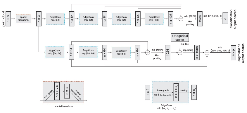
Fig. 14: DGCNN model architecture using EdgeConv [1]

Authors discover benefits of graph re-computation using nearest neighbors in the feature space. The key points of DGCNN can be summarized as follows —–

1. Design two different architectures for classification and segmentation tasks as depicted by two branches in figure 14.
2. Both architectures share a spatial transformer component, computing a global shape transformation.
3. The classification network includes two EdgeConv layers, followed by a pooling operation and three fully-connected layers producing classification output scores.
4. The segmentation network uses a sequence of three EdgeConv layers, followed by three fully-connected layers producing, for each point, segmentation output scores.
5. Each EdgeConv uses shared edge function, $h^{(l)}(x_i^{(l)}, x_j^{(l)}) = h^{(l)}(x_i^{(l)}, x_j^{(l)}-x_i^{(l)})$ across all layers and aggregation operation, $\square = max$
6. For the classification architecture, the graph is constructed using $k=20$ nearest neighbors, while $k=30$ in segmentation architecture.

Figure 11 shows the structure of the feature space produced at different stages of network architecture.

Fig. 11: Structure of feature space produced at different stages of network architecture. Visualized as the distance between the red point and the rest of the points. [1]

Evaluation

Models constructed using EdgeConv can be evaluated for three major tasks: classification, part segmentation, and semantic segmentation.

Classification Results

Authors evaluate their classification model based on the ModelNet40 [20] classification task. They follow the same strategy as PointNet. The hyper-parameters are as follow:

1. Optimizer: Adam [40]
2. Learning rate: 0.0001, reduced by factor 2 every 20 epochs
3. Decay rate for batch normalization: initially 0.5 and 0.99 finally
4. Batch size: 32
5. Momentum: 0.9

Figure 12 shows mean class accuracy and overall accuracy of different existing networks for classification on ModelNet40.

Fig. 12: Classification results on ModelNet40 [1]

Part Segmentation Results

EdgeConv model architectures are extended for part segmentation task on ShapeNet part dataset [41]. The same training setting is adapted from the classification task, except k is changed from 20 to 30 due to the increase of point density. NVIDIA TITAN X GPUs are used to maintain the training batch size in a distributed manner. The metric Intersection-over-Union (IoU) is used for the evaluation and comparison of the models. Figure 15 shows the results on ShapeNet part segmentation dataset.

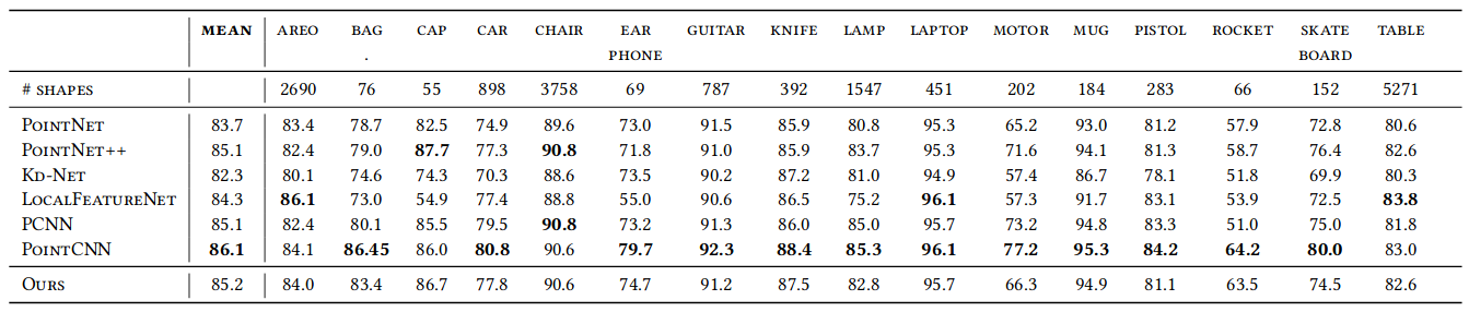
Fig. 15: Part segmentation results on ShapeNet part dataset. Metric is mIoU(%) on points. [1]

Semantic Scene Segmentation

Authors evaluate their model on Standford Large-Scale 3D Indoor Spaces Dataset (S3DIS) [42] for semantic scene segmentation task. The model used for this task is similar to the part segmentation model, except that a probability distribution over semantic object classes is generated for each input point. Figure 13 shows the results of 3D semantic segmentation task on S3DIS dataset by comparing existing models.

Fig. 13: 3D semantic segmentation results on S3DIS. MS+CU for multi-scale block features with consolidation units; G+RCU for the grid-blocks with recurrent consolidation Units. [1]

Later Work

There have been a lot of improvement and alternatives in the field of point clouds processing and graph convolutional neural networks since the paper published. PCNN [43] and URSA [44] are such two interesting works on point cloud data processing. PCNN employs an extension operator from surface functions to volumetric functions for the robustness of convolution and pooling operations. URSA uses a constellation of points to learn classification information from point cloud data.

Conclusion

The paper introduces a dynamic graph update for graph convolutional networks using EdgeConv operator. EdgeConv can be incorporated easily with any existing graph CNN architecture. A wide range of experiments proves their hypothesis and shows that consideration of local geometric features in 3d recognition tasks improves in the accuracy with a large margin. Authors wish to extend their work by designing a non-shared transformer network that works on each local patch differently. They would like to extend the applicability of dynamic graph CNN in more abstract point clouds i.e. data coming from document retrieval rather than 3D geometry.

References

[1] Y. Wang, Y. Sun, Z. Liu, S. E. Sarma, M. M. Bronstein, and J. M. Solomon, “Dynamic graph CNN for learning on point clouds,” CoRR, vol. abs/1801.07829, 2018. [Online]. Available: http://arxiv.org/abs/1801.07829

[2] C. R. Qi, H. Su, K. Mo, and L. J. Guibas, “Pointnet: Deep learning on point sets for 3d classification and segmentation,” CoRR, vol. abs/1612.00593, 2016. [Online]. Available: http://arxiv.org/abs/1612.00593

[3] C. R. Qi, L. Yi, H. Su, and L. J. Guibas, “Pointnet++: Deep hierarchical feature learning on point sets in a metric space,” CoRR, vol. abs/1706.02413, 2017. [Online]. Available: http://arxiv.org/abs/1706.02413

[4] “Point cloud — Wikipedia, the free encyclopedia.” [Online]. Available: https://en.wikipedia.org/wiki/Point_cloud

[5] “Adobe research.” [Online]. Available: https://research.adobe.com/news/a-papier-mache-approach-to-learning-3d-surface-generation

[6] “Mesh ploygon — Wikipedia, the free encyclopedia.” [Online]. Available: https://en.wikipedia.org/wiki/Polygon_mesh

[7] Y. Zhu, R. Mottaghi, E. Kolve, J. J. Lim, A. Gupta, L. Fei-Fei, and A. Farhadi, “Target-driven visual navigation in indoor scenes using deep reinforcement learning,” CoRR, vol. abs/1609.05143, 2016. [Online]. Available: http://arxiv.org/abs/1609.05143

[8] C. R. Qi, W. Liu, C. Wu, H. Su, and L. J. Guibas, “Frustum pointnets for 3d object detection from RGB-D data,” CoRR, vol. abs/1711.08488, [Online]. Available: http://arxiv.org/abs/1711.08488

[9] R. B. Rusu, Z.-C. Marton, N. Blodow, M. E. Dolha, and M. Beetz, “Towards 3d point cloud based object maps for household environments,” Robotics and Autonomous Systems, vol. 56, pp. 927–941, 2008.

[10] R. Schnabel, R. Wahl, R. Wessel, and R. Klein, “Shape recognition in 3d point-clouds,” 05 2012.

[11] O. V. Kaick, H. Zhang, G. Hamarneh, and D. Cohen-or, “A survey on shape correspondence,” 2011.

[12] Y. Guo, M. Bennamoun, F. Sohel, M. Lu, and J. Wan, “3d object recognition in cluttered scenes with local surface features: A survey,” IEEE Transactions on Pattern Analysis and Machine Intelligence, 04 2014.

[13] S. Biasotti, A. Cerri, A. M. Bronstein, and M. M. Bronstein, “Recent trends, applications, and perspectives in 3d shape similarity assessment,” Comput. Graph. Forum, vol. 35, pp. 87–119, 2016.

[14] Y. LeCun, B. Boser, J. S. Denker, D. Henderson, R. E. Howard, W. Hubbard, and L. D. Jackel, “Backpropagation applied to handwritten zip code recognition,” Neural Comput., vol. 1, no. 4, pp. 541–551, Dec. [Online]. Available: http://dx.doi.org/10.1162/neco.1989.1.4.541

[15] A. Krizhevsky, I. Sutskever, and G. E. Hinton, “Imagenet classification with deep convolutional neural networks,” Commun. ACM, vol. 60, no. 6, pp. 84–90, May 2017. [Online]. Available: http://doi.acm.org/10.1145/3065386

[16] “Convolutional neural networks — towards data science.” [Online]. Available: https://towardsdatascience.com/applied-deep-learning-part-4-convolutional-neural-networks-584bc134c1e2

[17] L. Wei, Q. Huang, D. Ceylan, E. Vouga, and H. Li, “Dense human body correspondences using convolutional networks,” CoRR, vol. abs/1511.05904, 2015. [Online]. Available: http://arxiv.org/abs/1511.05904

[18] H. Su, S. Maji, E. Kalogerakis, and E. G. Learned- Miller, “Multi-view convolutional neural networks for 3d shape recognition,” CoRR, vol. abs/1505.00880, 2015. [Online]. Available: http://arxiv.org/abs/1505.00880

[19] D. Maturana and S. Scherer, “Voxnet: A 3d convolutional neural network for real-time object recognition,” 2015 IEEE/RSJ International Conference on Intelligent Robots and Systems (IROS), pp. 922–928, 2015.

[20] Z. Wu, S. Song, A. Khosla, F. Yu, L. Zhang, X. Tang, and J. Xiao, “3d shapenets: A deep representation for volumetric shapes,” 06 2015, pp. 1912–1920.

[21] C. R. Qi, H. Su, M. Nießner, A. Dai, M. Yan, and L. J. Guibas, “Volumetric and multi-view cnns for object classification on 3d data,” CoRR, vol. abs/1604.03265, 2016. [Online]. Available: http://arxiv.org/abs/1604.03265

[22] M. Jaderberg, K. Simonyan, A. Zisserman, and K. Kavukcuoglu, “Spatial transformer networks,” CoRR, vol. abs/1506.02025, 2015. [Online]. Available: http://arxiv.org/abs/1506.02025

[23] Y. Li, R. Bu, M. Sun, and B. Chen, “Pointcnn,” CoRR, vol. abs/1801.07791, 2018. [Online]. Available: http://arxiv.org/abs/1801.07791

[24] Y. Shen, C. Feng, Y. Yang, and D. Tian, “Neighbors do help: Deeply exploiting local structures of point clouds,” CoRR, vol. abs/1712.06760, [Online]. Available: http://arxiv.org/abs/1712.06760

[25] M. M. Bronstein, J. Bruna, Y. LeCun, A. Szlam, and P. Vandergheynst, “Geometric deep learning: going beyond euclidean data,” CoRR, vol. abs/1611.08097, 2016. [Online]. Available: http://arxiv.org/abs/1611.08097

[26] J. Bruna, W. Zaremba, A. Szlam, and Y. Lecun, “Spectral networks and locally connected networks on graphs,” in International Conference on Learning Representations (ICLR2014), CBLS, April 2014, 2014.

[27] D. I. Shuman, S. K. Narang, P. Frossard, A. Ortega, and P. Vandergheynst, “Signal processing on graphs: Extending high-dimensional data analysis to networks and other irregular data domains,” CoRR, vol. abs/1211.0053, 2012. [Online]. Available: http://arxiv.org/abs/1211.0053

[28] M. Defferrard, X. Bresson, and P. Vandergheynst, “Convolutional neural networks on graphs with fast localized spectral filtering,” CoRR, vol. abs/1606.09375, 2016. [Online]. Available: http://arxiv.org/abs/1606.09375

[29] T. N. Kipf and M. Welling, “Semi-supervised classification with graph convolutional networks,” CoRR, vol. abs/1609.02907, 2016. [Online]. Available: http://arxiv.org/abs/1609.02907

[30] R. Levie, F. Monti, X. Bresson, and M. M. Bronstein, “Cayleynets: Graph convolutional neural networks with complex rational spectral filters,” CoRR, vol. abs/1705.07664, 2017. [Online]. Available: http://arxiv.org/abs/1705.07664

[31] L. Yi, H. Su, X. Guo, and L. J. Guibas, “Syncspeccnn: Synchronized spectral CNN for 3d shape segmentation,” CoRR, vol. abs/1612.00606, [Online]. Available: http://arxiv.org/abs/1612.00606

[32] J. Masci, D. Boscaini, M. M. Bronstein, and P. Vandergheynst, “Shapenet: Convolutional neural networks on non-euclidean manifolds,” CoRR, vol. abs/1501.06297, 2015. [Online]. Available: http://arxiv.org/abs/1501.06297

[33] J. Zhou, G. Cui, Z. Zhang, C. Yang, Z. Liu, and M. Sun, “Graph neural networks: A review of methods and applications,” CoRR, vol. abs/1812.08434, 2018. [Online]. Available: http://arxiv.org/abs/1812.08434

[34] “Graph convolutional networks: Neighbourhood aggregation.” [Online]. Available: http://snap.stanford.edu/proj/embeddings-www/

[35] A. Loukas and P. Vandergheynst, “Spectrally approximating large graphs with smaller graphs,” CoRR, vol. abs/1802.07510, 2018. [Online]. Available: http://arxiv.org/abs/1802.07510

[36] I. Safro, P. Sanders, and C. Schulz, “Advanced coarsening schemes for graph partitioning,” CoRR, vol. abs/1201.6488, 2012. [Online]. Available: http://arxiv.org/abs/1201.6488

[37] “Max pooling —– computer science wiki.” [Online]. Available: https://computersciencewiki.org/index.php/Max-pooling_/_Pooling)

[38] M. Defferrard and P. Vandergheynst, “Convolutional neural networks on graphs with fast localized spectral filtering,” Advances in Neural Information Processing Systems, 2016.

[39] Z. Wu, S. Pan, F. Chen, G. Long, C. Zhang, and P. S. Yu, “A comprehensive survey on graph neural networks,” CoRR, vol. abs/1901.00596, 2019. [Online]. Available: http://arxiv.org/abs/1901.00596

[40] D. Kingma and J. Ba, “Adam: A method for stochastic optimization,” International Conference on Learning Representations, 12 2014.

[41] L. Yi, V. G. Kim, D. Ceylan, I.-C. Shen, M. Yan, H. Su, C. Lu, Q. Huang, A. Sheffer, and L. Guibas, “A scalable active framework for region annotation in 3d shape collections,” ACM Trans. Graph., vol. 35, no. 6, pp. 210:1–210:12, Nov. 2016. [Online]. Available: http://doi.acm.org/10.1145/2980179.2980238

[42] I. Armeni, O. Sener, A. R. Zamir, H. Jiang, I. K. Brilakis, M. Fischer, and S. Savarese, “3d semantic parsing of large-scale indoor spaces,” 2016 IEEE Conference on Computer Vision and Pattern Recognition (CVPR), pp. 1534–1543, 2016.

[43] M. Atzmon, H. Maron, and Y. Lipman, “Point convolutional neural networks by extension operators,” CoRR, vol. abs/1803.10091, 2018. [Online]. Available: http://arxiv.org/abs/1803.10091

[44] M. B. Skouson, “URSA: A neural network for unordered point clouds using constellations,” CoRR, vol. abs/1808.04848, 2018. [Online]. Available: http://arxiv.org/abs/1808.04848