Time Series Analysis in Python - Introduction to ARIMA

What is Time Series?

If we want to predict something in future i.e. stock prices, sales etc, we use time series analysis over past data. We can predict daily stock price, weekly interest rates, sales figure etc where the outcome varies over time. In such scenarios, we use time series forecasting.

A time series is a set of observation taken at specified times usually at equal intervals. It is used to predict future values based on the previously observed values.

By time series analysis we not only predict the future values but also able to understand past behavior, plan for the future and evaluate current accomplishment.

Componets of Time Series

• Trend:

  • A trend exists when there is a long-term increase or decrease in the data. It does not have to be linear. It could go from an increasing trend to a decreasing trend.
  • There is a trend in the antidiabetic drug sales data shown below.

Source: otext.org

• Seasonality:

  • A seasonal pattern occurs when a time series is affected by seasonal factors such as the time of the year or the day of the week.
  • Seasonality is always of a fixed and known frequency.
  • The monthly sales of antidiabetic drugs above show seasonality which is induced partly by the change in the cost of the drugs at the end of the calendar year.

• Irregularity:

  • It is also called residual.
  • These are erratic in nature, unsystematic, basically happens for short durations and not repeating.
  • Let’s take an example. If there is a sudden natural disaster i.e flood in a town out of nowhere, a lot of people buy medicine and ointment and after sometime when everything settles down, sales of those ointments might go down. Nobody knows how many numbers of sales are going to happen that time and also cannot force the event not to happen. These type of random variations are called irregularity.

• Cyclic:

  • A cycle occurs when the data exhibit rises and falls that are not of a fixed frequency.
  • These fluctuations are usually due to economic conditions, and are often related to the “business cycle”. The duration of these fluctuations is usually at least 2 years.

When NOT to use Time Series?

Time series is not applicable when-

1. values are constant such as y = c.
2. values are in the form of a function, such as y = sin(x), y = log(x).

What is Stationarity?

• Time series has a particular behavior over time, there is a very high probability that it will follow the same in the future.
• A stationary time series is one whose properties do not depend on the time at which the series is observed.
• Time series with trends (varying mean over time), or with seasonality (variations of a specific time frame), are not stationary — the trend and seasonality will affect the value of the time series at different times.
• On the other hand, a white noise series is stationary — it does not matter when you observe it, it should look much the same at any point in time.
• Some cases can be confusing — a time series with cyclic behavior (but with no trend or seasonality) is stationary. This is because the cycles are not of a fixed length, so before we observe the series we cannot be sure where the peaks and troughs of the cycles will be.

In general, a stationary time series will have no predictable patterns in the long-term. Time plots will show the series to be roughly horizontal (although some cyclic behavior is possible), with constant variance.

Figure 2: Which of these series are stationary? (a) Google stock price for 200 consecutive days; (b) Daily change in the Google stock price for 200 consecutive days; (c) Annual number of strikes in the US; (d) Monthly sales of new one-family houses sold in the US; (e) Annual price of a dozen eggs in the US (constant dollars); (f) Monthly total of pigs slaughtered in Victoria, Australia; (g) Annual total of lynx trapped in the McKenzie River district of north-west Canada; (h) Monthly Australian beer production; (i) Monthly Australian electricity production. Source: otext.org

Consider the nine series plotted in Figure 2. Which of these do you think are stationary?

Obvious seasonality rules out series (d), (h) and (i). Trends and changing levels rules out series (a), (c), (e), (f) and (i). Increasing variance also rules out (i). That leaves only (b) and (g) as stationary series.

At first glance, the strong cycles in series (g) might appear to make it non-stationary. But these cycles are aperiodic. In the long-term, the timing of these cycles is not predictable. Hence the series is stationary.

How to Remove Stationarity?

Following characteristics can be found in stationary time series. We have to get rid of those characteristics.

• Constant means according to the time
• Constant variance at different time intervals
• Autocovariance that does not depend on time i.e. correlation between values of any time interval t and their previous time intervals such as t-1, t-2 etc.

Tests to Check Stationarity

1. Rolling Statistics

   • Plot the moving average or moving variance and see if it varies with time.
   • It’s more of a visual technique, not suitable for production.
   • It can be used as POC (proof of concept) purpose.

2. ADCF (Augmented Dickey-Fuller) Test

   • The test starts with a null hypothesis that states that the time series is non-stationary, followed by some statistical results based on the hypothesis.
   • The test results comprise of a Test Statistic Value and some Critical Values.
   • We will go the rules that check stationarity in a time series later on in our example.
   • More about this algorithm can be found here.

What is the ARIMA model?

• ARIMA stands for Auto-Regressive Integrated Moving Average
• ARIMA is one of the best models to work with time series data.
• Combination of two models, AR and MA
• AR (Auto-Regressive) model: Correlation between data in previous time steps and current time step. Parameterized with p, called autoregressive lags term.
• MA (Moving Average) model: Moving average to smoothen data and average the noises and irregularities. Parameterized with q, called moving average term.
• These two models are then integrated with a degree of differencing from previous p time intervals.

ACF and PACF

To find p and q, we have to determine PACF and ACF which are autocorrelation function and partial autocorrelation function respectively of a time series. ACF is used to find autocorrelation between timestamp t and t-k where k = 1, 2, …, t-1. This allows the model to predict according to the trend. Again, PACF is also determined for the same purpose but over residuals to smoothen out noises.

If you are interested to know some details of ACF and PACF, please refer to this link.

Example: Forecast Future

Build a model to forecast the demand or passenger traffic in airplanes. The data is classified in date/time and the passengers traveling per month.

Import necessary libraries

We will be using numpy for matrix manipulation, pandas for loading dataset from csv, matplotlib to visualize some data in different formats i.e. graphs, charts etc. Also, we will be using some other libraries to perform statistical analysis later on.

1
2
3
4
5
6
7

import numpy as np
import pandas as pd
import matplotlib.pylab as plt
%matplotlib inline

from matplotlib.pylab import rcParams
rcParams['figure.figsize'] = 10, 61

Load the dataset air-passengers.csv

First, we need to convert date strings as python date time format. Also, we want to select Month as the index of this data table.

1
2
3
4

dataset = pd.read_csv('data/air-passengers.csv')
# parse strings to datetime type
dataset['Month'] = pd.to_datetime(dataset['Month'], infer_datetime_format=True)
indexed_data = dataset.set_index(['Month'])

Let’s print some data from the beginning of the table.

1

indexed_data.head(5)

Let’s plot this data as a graph with matplotlib.

1
2
3
4
5

## plot graph

plt.xlabel("Date")
plt.ylabel("#Passengers")
plt.plot(indexed_data)

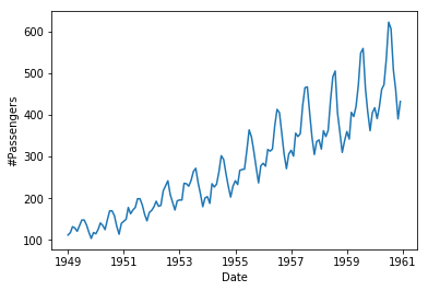
Check if the data is Stationary or not

We will be using both rolling statistics and ADCF test for this purpose.

Determining Rolling Statistics

Since the dataset is monthly, we can set the rolling window as yearly (12 months), half-yearly (6 months) or even quarterly (4 months). We will be using 12 months or 12 rows for this case to determine the means, standard deviations and check if they are constant or not.

1
2
3
4
5
6

# Determining rolling statistics

rolling_mean = indexed_data.rolling(window=12).mean()
rolling_std = indexed_data.rolling(window=12).std()

print rolling_mean, rolling_std

 1
 2
 3
 4
 5
 6
 7
 8
 9
10
11
12
13
14
15
16
17
18
19
20
21
22
23
24
25
26
27
28
29
30
31
32
33
34
35
36
37
38
39
40
41
42
43
44
45
46
47
48
49
50
51
52
53
54
55
56
57
58
59
60
61
62
63
64
65

Month #Passengers
1949-01-01          NaN
1949-02-01          NaN
1949-03-01          NaN
1949-04-01          NaN
1949-05-01          NaN
1949-06-01          NaN
1949-07-01          NaN
1949-08-01          NaN
1949-09-01          NaN
1949-10-01          NaN
1949-11-01          NaN
1949-12-01   126.666667
1950-01-01   126.916667
1950-02-01   127.583333
1950-03-01   128.333333
1950-04-01   128.833333
1950-05-01   129.166667
1950-06-01   130.333333
1950-07-01   132.166667
1950-08-01   134.000000
1950-09-01   135.833333
1950-10-01   137.000000
1950-11-01   137.833333
1950-12-01   139.666667
1951-01-01   142.166667
1951-02-01   144.166667
1951-03-01   147.250000
1951-04-01   149.583333
1951-05-01   153.500000
1951-06-01   155.916667
...                 ...
1958-07-01    59.590013
1958-08-01    65.557054
1958-09-01    65.557054
1958-10-01    65.106207
1958-11-01    64.593074
1958-12-01    64.530472
1959-01-01    63.627229
1959-02-01    61.759553
1959-03-01    61.597422
1959-04-01    60.284678
1959-05-01    60.008270
1959-06-01    63.009138
1959-07-01    71.987951
1959-08-01    80.049369
1959-09-01    81.485451
1959-10-01    79.680422
1959-11-01    74.498729
1959-12-01    69.830097
1960-01-01    66.624399
1960-02-01    61.866180
1960-03-01    61.382741
1960-04-01    60.171472
1960-05-01    60.184565
1960-06-01    65.021849
1960-07-01    77.194510
1960-08-01    83.630500
1960-09-01    84.617276
1960-10-01    82.541954
1960-11-01    79.502382
1960-12-01    77.737125

[144 rows x 1 columns]

We will see that the first 11 rows have NaN values. We took means and standard deviations over every 12 rows from the beginning. Since these rows don’t fulfill the rolling window, we have got data starting from the 12th row.

Let’s plot these rolling statistics.

1
2
3
4
5
6
7
8

# Plot rolling statistics

orig = plt.plot(indexed_data, color='blue', label='Original')
mean = plt.plot(rolling_mean, color='red', label='Rolling Mean')
std = plt.plot(rolling_std, color='black', label='Rolling Std')
plt.legend(loc='best')
plt.title('Rolling Mean & Standard Deviation')
plt.show(block=False)

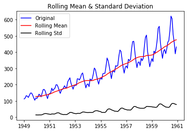
We can see that the means and standard deviations are not constant and we can say that this time series is not stationary.

Perform Dicky-Fuller Test

We will be using statsmodels library for this purpose. The adfuller test will give us the following data-

• Test Statistic
• p-value
• Number of lags used
• Number of observations used

If we don’t want to dive into the details of Dicky-Fuller algorithm and just want to know whether the time series is stationary or not from this test results, then we can see the summary of the algorithm below-

• If
  • p-value > 0.05: The data is non-stationary.
  • p-value <= 0.05: The data is stationary.
• If
  • test statistic value is significantly less than critical values (possibly less than 1% of critical values): The data is stationary.
  • test statistic value is greater than critical values: The data is non-stationary.

 1
 2
 3
 4
 5
 6
 7
 8
 9
10
11
12
13

# Perform Dicky-Fuller test

from statsmodels.tsa.stattools import adfuller

print 'Result of Dicky=Fuller Test'
dftest = adfuller(indexed_data['#Passengers'], autolag='AIC')

dfoutput = pd.Series(dftest[0:4], index=['Test Statistic', 'p-value', '#Lags Used', '#Observations Used'])

for key, value in dftest[4].items():
    dfoutput['Critical Value (%s)'%key] = value

print(dfoutput)

1
2
3
4
5
6
7
8
9

Result of Dicky=Fuller Test
Test Statistic            0.815369
p-value                   0.991880
#Lags Used               13.000000
#Observations Used      130.000000
Critical Value (5%)      -2.884042
Critical Value (1%)      -3.481682
Critical Value (10%)     -2.578770
dtype: float64

In summary, we can say that the data is non-stationary since from adfuller test we can see that p-value is greater than 0.05 and statistic value is greater than critical values.

Formalize Stationarity Checking in a Function

We can now formalize the stationarity checking scripts using a function test_stationarity. We will perform both rolling statistics and ADFC test to check stationarity.

 1
 2
 3
 4
 5
 6
 7
 8
 9
10
11
12
13
14
15
16
17
18
19
20
21
22

from statsmodels.tsa.stattools import adfuller
def test_stationarity(timeseries):

    # Determinign rolling statistics
    rolling_mean = timeseries.rolling(window=12).mean()
    rolling_std = timeseries.rolling(window=12).std()

    # Plot rolling statistics

    orig = plt.plot(timeseries, color='blue', label='Original')
    mean = plt.plot(rolling_mean, color='red', label='Rolling Mean')
    std = plt.plot(rolling_std, color='black', label='Rolling Std')
    plt.legend(loc='best')
    plt.title('Rolling Mean & Standard Deviation')
    plt.show(block=False)

    print 'Result of Dicky=Fuller Test'
    dftest = adfuller(timeseries['#Passengers'], autolag='AIC')
    dfoutput = pd.Series(dftest[0:4], index=['Test Statistic', 'p-value', '#Lags Used', '#Observations Used'])
    for key, value in dftest[4].items():
        dfoutput['Critical Value (%s)'%key] = value
    print(dfoutput)

Make The Data Stationary

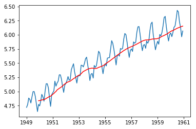
There are several ways to make the data stationary, but it totally depends on the data. For this case, we can take the log scale data and subtract moving average from that to make it somewhat stationary.

1
2
3
4
5
6
7
8

# Estimating trend

indexed_data_log_scale = np.log(indexed_data)
moving_average = indexed_data_log_scale.rolling(window=12).mean()
moving_std = indexed_data_log_scale.rolling(window=12).mean()

plt.plot(indexed_data_log_scale)
plt.plot(moving_average, color='red')

1
2
3

dataset_log_scale_minus_moving_average = indexed_data_log_scale - moving_average
dataset_log_scale_minus_moving_average.dropna(inplace=True)
dataset_log_scale_minus_moving_average.head(12)

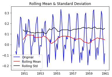
Now call this function with our newly transformed data.

1

test_stationarity(dataset_log_scale_minus_moving_average)

1
2
3
4
5
6
7
8

Result of Dicky=Fuller Test
Test Statistic           -3.162908
p-value                   0.022235
#Lags Used               13.000000
#Observations Used      119.000000
Critical Value (5%)      -2.886151
Critical Value (1%)      -3.486535
Critical Value (10%)     -2.579896

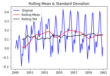
This is better than original and looks little bit stationary and adfuller test also suggests that this transformed series is stationary. Let’s do some other type of transformations to make it more stationary. We can start with subtracting exponentially weighted average from log scaled values and check again its stationarity.

1
2
3

dataset_log_scale_ewm = indexed_data_log_scale.ewm(halflife=12, min_periods=0, adjust=True).mean()
dataset_log_scale_minus_ewm = indexed_data_log_scale - dataset_log_scale_ewm
test_stationarity(dataset_log_scale_minus_ewm)

1
2
3
4
5
6
7
8

Result of Dicky=Fuller Test
Test Statistic           -3.601262
p-value                   0.005737
#Lags Used               13.000000
#Observations Used      130.000000
Critical Value (5%)      -2.884042
Critical Value (1%)      -3.481682
Critical Value (10%)     -2.578770

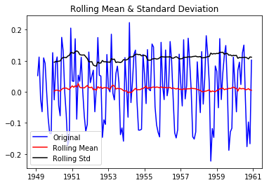
So both of the above transformations can make the data stationary. Now let’s start working on finding p, d and q to feed in our ARIMA model.

First of all, let’s get first order differences.

1
2
3

dataset_log_first_order_diff = indexed_data_log_scale - indexed_data_log_scale.shift()
dataset_log_first_order_diff.dropna(inplace=True)
test_stationarity(dataset_log_first_order_diff)

1
2
3
4
5
6
7
8

Result of Dicky=Fuller Test
Test Statistic           -2.717131
p-value                   0.071121
#Lags Used               14.000000
#Observations Used      128.000000
Critical Value (5%)      -2.884398
Critical Value (1%)      -3.482501
Critical Value (10%)     -2.578960

Decompose into Trend, Seasonality and Residual

Now, let’s decompose values into the trend, seasonal and residual components. We can do so using statsmodels.tsa.seasonal package.

 1
 2
 3
 4
 5
 6
 7
 8
 9
10
11
12
13
14
15
16
17
18
19
20
21
22
23

from statsmodels.tsa.seasonal import seasonal_decompose
decomposition = seasonal_decompose(indexed_data_log_scale)

trend = decomposition.trend
seasonal = decomposition.seasonal
residual = decomposition.resid

plt.subplot(411)
plt.plot(indexed_data_log_scale, label='Original')
plt.legend(loc='best')

plt.subplot(412)
plt.plot(trend, label='Trend')
plt.legend(loc='best')

plt.subplot(413)
plt.plot(seasonal, label='Seasonality')
plt.legend(loc='best')

plt.subplot(414)
plt.plot(residual, label='Residuals')
plt.legend(loc='best')
plt.tight_layout()

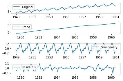
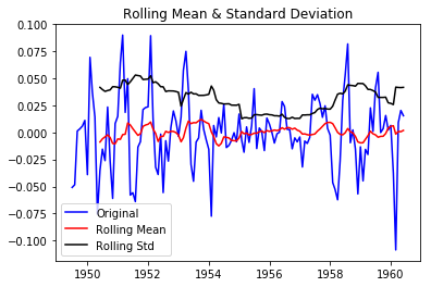
Now, we can test that if the residual is stationary or not using our test_stationarity functiuon.

1
2
3

decomposed_log_data = residual
decomposed_log_data.dropna(inplace=True)
test_stationarity(decomposed_log_data)

1
2
3
4
5
6
7
8
9

Result of Dicky=Fuller Test
Test Statistic         -6.332387e+00
p-value                 2.885059e-08
#Lags Used              9.000000e+00
#Observations Used      1.220000e+02
Critical Value (5%)    -2.885538e+00
Critical Value (1%)    -3.485122e+00
Critical Value (10%)   -2.579569e+00
dtype: float64

We can easily say that the residual is not stationary. Since MA component deals with residual, we have to transform this data to make it stationary, so that it smoothen it out to predict what will happen next. But for now, don’t worry about that since ACF and PACF curves will help us to find proper values of p and q, and feeding those into the ARIMA model will do the job for us.

Determine ACF and PACF

Now, we know the value of d. We have to calculate the values of p and q. We can find these values from ACF and PACF graph. Let’s plot those graph.

 1
 2
 3
 4
 5
 6
 7
 8
 9
10
11
12
13
14
15
16
17
18
19
20
21
22

# ACF and PACF plots|:
from statsmodels.tsa.stattools import acf, pacf

lag_acf = acf(dataset_log_first_order_diff, nlags=20)
lag_pacf = pacf(dataset_log_first_order_diff, nlags=20, method='ols')

# Plot ACF
plt.subplot(121)
plt.plot(lag_acf)
plt.axhline(y=0, linestyle='--', color='gray')
plt.axhline(y=-1.96/np.sqrt(len(dataset_log_first_order_diff)), linestyle='--', color='gray')
plt.axhline(y=1.96/np.sqrt(len(dataset_log_first_order_diff)), linestyle='--', color='gray')
plt.title('ACF')

# Plot PACF
plt.subplot(122)
plt.plot(lag_pacf)
plt.axhline(y=0, linestyle='--', color='gray')
plt.axhline(y=-1.96/np.sqrt(len(dataset_log_first_order_diff)), linestyle='--', color='gray')
plt.axhline(y=1.96/np.sqrt(len(dataset_log_first_order_diff)), linestyle='--', color='gray')
plt.title('PACF')
plt.tight_layout()

In order to calculate p and q, we have to check what is the value that cuts off its origin for the first time. Looking at PACF curve, we can see that at the time around 2, the first time curve cuts the horizontal axis, hence the value of p is 2 and similarly from ACF curve, we find that the value of q is also around 2.

Feed p, d, and q into ARIMA Model

We have found the values of p, d, and q, which are 2, 1 and 2 respectively. Let’s fit our ARIMA model with these values.

1
2
3
4
5
6
7
8

from statsmodels.tsa.arima_model import ARIMA

#ARIMA Model
model = ARIMA(indexed_data_log_scale, order=(2, 1, 2))
results_ARIMA = model.fit(disp=-1)
plt.plot(dataset_log_first_order_diff)
plt.plot(results_ARIMA.fittedvalues, color='red')
plt.title('RSS: %.4f'% sum((results_ARIMA.fittedvalues-dataset_log_first_order_diff['#Passengers'])**2))

1

Text(0.5,1,'RSS: 1.0292')

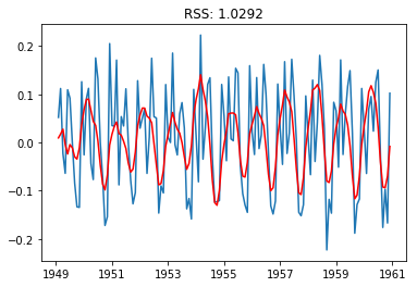
Check If Fitted Values Depicts Original Curve

Since we are working with first-order differences, we have to covert fitted values back to the real values. We went through the following sequence from given values to fitted values:

1. Take logarithm of the values
2. Take first-order differences of the values found in step no 1

So we have to reverse the process to predict the next values:

1. Get back the first item from the log scaled values and place it at index 0 after shifting the fitted values once
2. Take cumulative sum to get back logarithm scaled values
3. Take exponentials of the values found in step no 2

1
2
3
4
5
6
7
8
9

# Get back to the state before differening
predictions_ARIMA_log = pd.Series(indexed_data_log_scale.loc[indexed_data_log_scale.index[0]].append(results_ARIMA.fittedvalues).cumsum(), index=indexed_data_log_scale.index)

# Get exponetials
predictions_ARIMA = np.exp(predictions_ARIMA_log)

# Plot predicted data vs original data
plt.plot(indexed_data)
plt.plot(predictions_ARIMA)

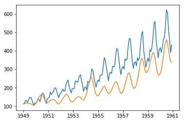
If we don’t want to be bothered about all these conversions, well, we have a piece of good news. ARIMA model also can plot the fitted values efficiently, even for future time intervals.

Predict and Plot Future Values Using The ARIMA Model

Now, our dataset has 144 rows, that means 12 years’ values. If we want to plot the graph for next 1 year, we have to call plot_predict() function from ARIMA model with parameters 1 (start from the first row) and 204 (first 144 + new 5x12=60 rows).

1

results_ARIMA.plot_predict(1,204)

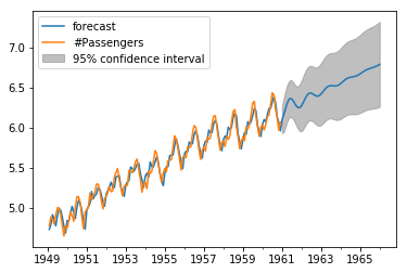
The forecast function from ARIMA model with parameter steps=60 will give us the new 60 values.

1
2

future = results_ARIMA.forecast(steps=60)
print np.exp(future[1])

 1
 2
 3
 4
 5
 6
 7
 8
 9
10

[1.08746262 1.11348487 1.12264437 1.12415063 1.12415874 1.12461435
 1.12481942 1.12500462 1.12776932 1.13582632 1.14879044 1.16321524
 1.1753643  1.18334355 1.1874086  1.18900856 1.18956455 1.18988252
 1.19041521 1.1917625  1.1946837  1.19956286 1.2059434  1.21268138
 1.21858755 1.22299943 1.22591873 1.22776853 1.22906372 1.23024086
 1.23166843 1.23368207 1.23651561 1.24016542 1.24433566 1.2485496
 1.25236108 1.2555239  1.25803132 1.26004567 1.26179869 1.26352486
 1.26543139 1.26767321 1.27031559 1.27330434 1.27647669 1.2796205
 1.2825529  1.28517677 1.28749351 1.28957958 1.29155007 1.29352656
 1.29561291 1.29787521 1.30032659 1.30292387 1.30558205 1.30820345]

If you are looking for the full working code, here it is.

Acknowledgement: I took help from several popular online blogs and video tutorials like simplilearn, edureka, machinelearningmastery, otext, just to name a few. I rephrased some sentences and would like to give them full credits.